Diversification
– Weighted
Performance
Evaluation
Investors hold diversification, long a bedrock of investor prudence, in high esteem. This is curious, as diversification is both ubiquitous and misunderstood. Diversification is typically associated with asset allocation, but fundamentally, diversification is a weighting strategy. We have formalized Diversification Weighted Performance Evaluation.
DIVERSIFICATION– WEIGHTED PERFORMANCE EVALUATION
Investors hold diversification, long a bedrock of investor prudence, in high esteem. This is curious, as diversification is both ubiquitous and misunderstood. Diversification is typically associated with asset allocation, but fundamentally, diversification is a weighting strategy. We have formalized diversification as a weighting approach.

A new approach to building a portfolio
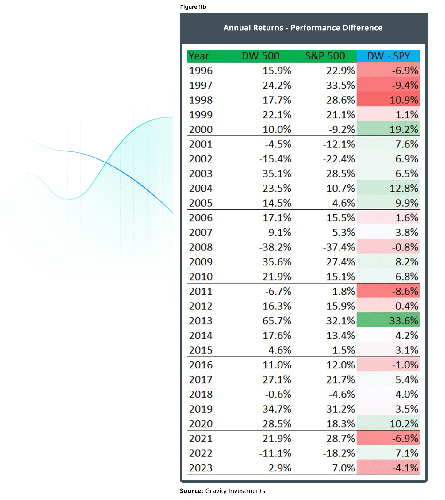
Using the components of the S&P 500 Index, we investigate an alternative, process-driven methodology for index construction and optimization called Diversification Weighting. We find that when reconstituting the S&P 500 universe from January 1996 through May 2014, using Diversification Optimization, we achieved annualized outperformance of 427 basis points against the capital-weighted benchmark, and achieved favorable results when compared against other weighted approaches applied to the same investments universe. We also introduce diversification measurement for context and clarity underpinning Diversification Optimization.
2023 Update and Revision:
In May 2023, this research was updated through April 4th, 2023. We have left all of the text the same, including any references to performance in the text. However, the majority of the charts and graphics have been updated. Notes on the update and revision are available on request. This brings the analysis to 27 years and the performance of the Diversification Weighted Strategy outperforms the Capitalization weighted strategy by 3.83% per year, net estimated fees and expenses.
Overview
Investors hold diversification, long a bedrock of investor prudence, in high esteem. This is curious, as diversification is both ubiquitous and misunderstood. Diversification is typically associated with asset allocation, but fundamentally, diversification is a weighting strategy. We have formalized diversification as a weighting approach. We believe Diversification Weighting is both unique and often superior to conventional weighting approaches. Importantly, it is not constrained to a particular market, style or even asset class.
In addition, we show portfolio diversification to provide material performance improvements to both risk and return. Part of the attraction to smart-beta euphoria is an intuition that repeatable investment performance is systematic. Investors prefer a repeatable process and especially a process rooted in things that are rather simple and easily understood.
Diversification as a concept has been around for a long time, but only in vague or indefinite terms. This paper describes various inventions for diversification measurement, visualization, and optimization, but a full treatment of all of these topics is beyond the scope of this article. The question we mean to address here is, does diversification work?
In essence, diversification increases for every equally weighted, uncorrelated asset added to a portfolio. When we put the portfolio in a geometric space, such additions add a dimension, which may measure the diversification therein. When we weight assets in a manner consistent with maximizing the portfolio dimensionality, perhaps subject to a utility function, the portfolio is said to be diversification-weighted.
table of Contents
Defining Diversification: The Framework
For Measurement And Optimization
For something to be optimized, it must have a clear and definable objective function. Diversification, while ethereal by its nature, can be defined with precision and definiteness.
For readers interested in diversification or how the results are obtained, we need to set some foundations in geometric modeling. The ensuing geometric modeling framework provides the background for both diversification measurement and optimization.
Asset correlations are measured, and assets are projected into a space that maps the measured correlations to the angles separating one asset from another so that assets with higher correlations have a more acute angle separating the vectors. Assets sharing zero correlation are mapped to a 90° angle, and assets with a -1 correlation are mapped as diametric opposites having a 180° angle.
Imagine a three-asset portfolio; each asset has zero correlation to the other two assets. Each asset takes the portfolio in a new direction. Note that all available dimensions are used as degrees of freedom to convey the relativity of the assets. It is a correlation in every dimension. We refer to this as having a relativity domain space. Imagine that we introduce a fourth uncorrelated asset. Where would it fit? It cannot fit in 3-D without creating some distortion. There is not enough dimensionality to hold it. We need to introduce an additional dimension, which may accurately represent the fourth uncorrelated asset.
In mathematics, there is no limit to dimensionality. So it is with portfolios. Diversification has no upper boundary; there can always be more. Any portfolio has an ambient dimensionality equal to the number of assets in it. The ambient dimension compacts with the spanning dimension after ringing out all of the redundant information caused by disparate weighting and positive correlations. The spanning dimension thus contains all of the portfolio’s information. It is a bit like a.jpeg at 100 percent quality. The dimension of the portfolio can be further reduced when associated with a confidence interval, such that it captures X percent of the portfolio. That dimensionality is called an “effective dimension.” It is like viewing a.jpeg at 90 percent quality; it captures the essence of the image but does not require the same amount of data. Thus, the lowest dimensions 1, 2, and 3 are the most pervasive and measure systematic diversification and risk exposure.
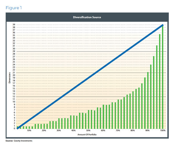
When we arrange the dimensions from the most pervasive or fundamental to the least, we can visualize the portfolio’s exposure across the dimensions. The vertical axis in Figure 1 gives the dimensions required to contain X percent of the portfolio.
This framework explains how portfolios sprawl across multiple dimensions. The primary dimensions give the systematic exposure on the left and it integrates with the idiosyncratic exposures on the right. Each new dimension acts as a source of diversification unto the portfolio. The blue shadow line gives the investor an understanding of what perfect diversification (given the investment quantity) would look like. The portfolio would mimic
this line if each asset were equally weighted and uncorrelated. The more exponential the portfolio graph, the greater the risk, as such exponential graphs are indicative of superficial diversification in asset quantity only.
We apply this diversification framework to weighted as well as unweighted portfolios. When the portfolio is already weighted, the framework gives the measurements of diversification as well as the visualization.
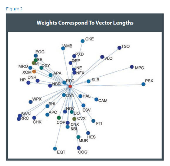
When the framework is applied to a weighted portfolio, the given weights for each asset are modeled as the vector lengths for each asset. Intuitively, the weight extends the assets in its given direction (Figure 2).
In essence, it is like a multidimensional pie chart containing relativity data.
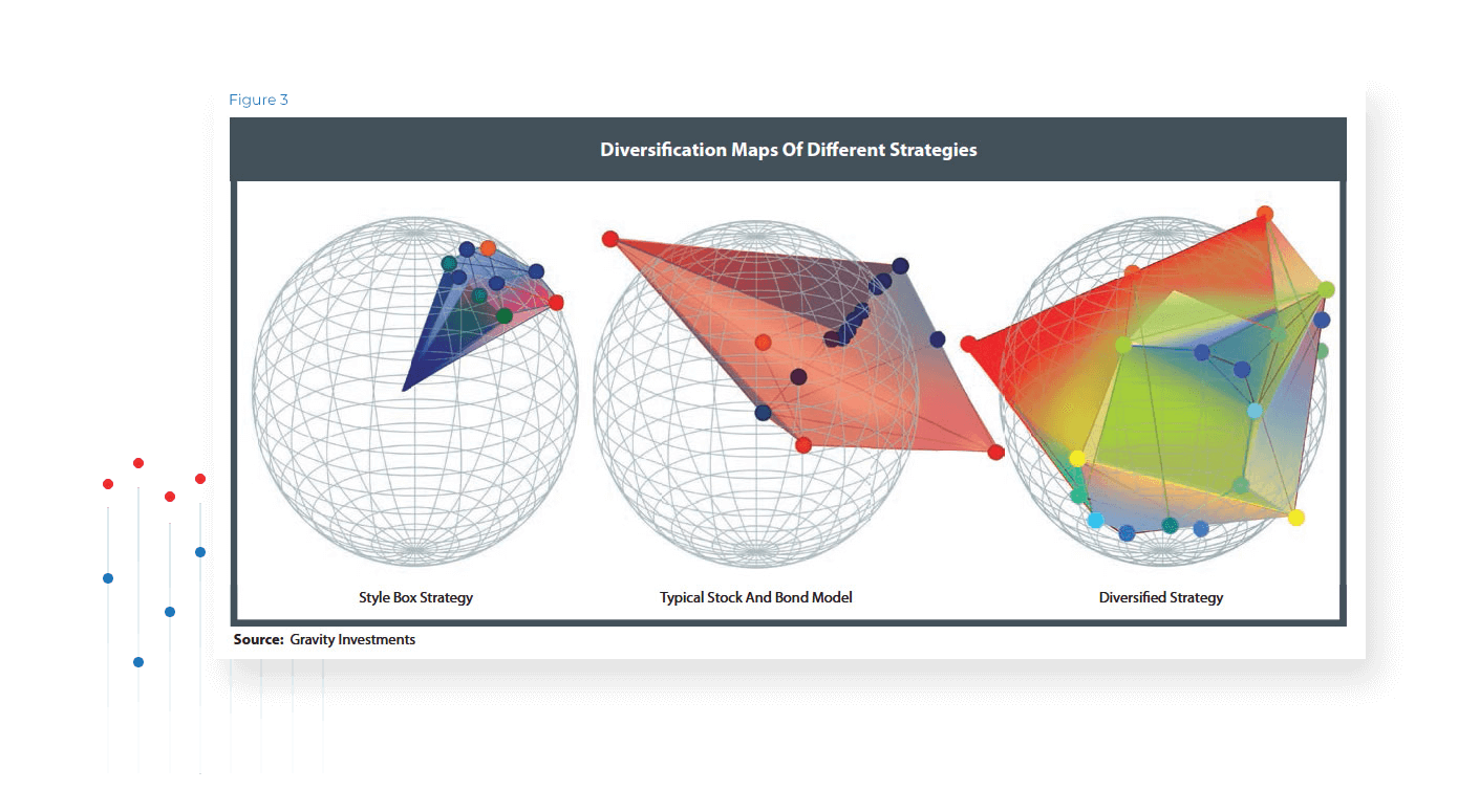
The resulting level of symmetry induced by the model structured by the assets’ weights and relationships provides a visual explanation of portfolio diversification. Portfolio balance is manifest as three-dimensional balance in the True Diversification model framework. True Diversification accounts for the diversification directly and captures both the systematic and nonsystematic perspectives (Figure 3). This process can be applied to any asset or any mix of assets, including disparate assets classes, or mixing of various instruments. We recycle this geometric modeling process to optimize diversification.
Diversification Optimization:
The Theoretical Foundation
The following section explains the general approaches of Diversification Optimization. Diversification Optimization is built on the same geometric framework for diversification visualization and measurement. The crucial difference is that the length of each asset’s vector is not its current weight in the portfolio, but a utility function.
The utility function is conventionally a risk-adjusted return. The utility function concept is very flexible; we have used metrics such as Sharpe ratios, Calmar ratios, total returns, fundamental scores, omega functions, and alphas. Assets with superior performance have longer vectors, literally extending the portfolio in its given direction. The choice of a utility function measures the relative attractiveness of the assets.
The portfolio thus has two elementary inputs: the relationship of each asset to every other asset in the portfolio, as measured by its correlation matrix and modeled by the relative angles; and the utility function for every asset measuring the relative attractiveness of each asset and modeling the magnitude of each vector. These are the only inputted asset variables.
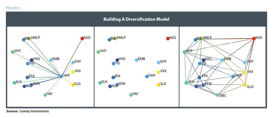
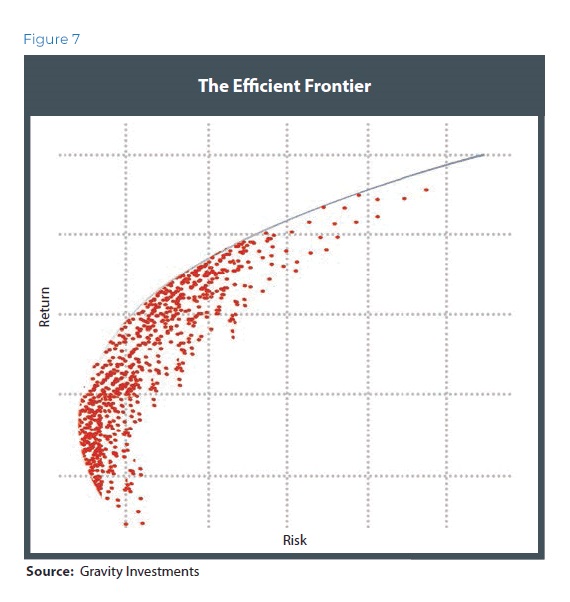
From this, we gather a point cloud of coordinate data and apply a convex hull about that point cloud. The hull is similar to the efficient frontier, except instead of 2-D it is 3-D, and the concept of efficiency is not mean-variance efficient, but diversification-utility efficient. Vector angles and lengths give the coordinates for the point cloud that creates the diversification frontier (Figure 4).
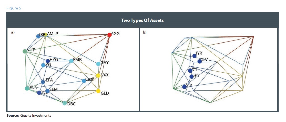
As Figure 5 shows, there are two types of assets: those that combine to create the frame (a) and those trapped inside (b). Efficient assets grow the portfolio in their respective directions. The interior assets are doing an inefficient job of growing the portfolios in their respective direction and are dominated by the assets comprising the diversification frontier. Interior assets are inefficient and normally discarded unless subject to a constraint.
While the 3-D graphics are useful for understanding the structure of the portfolio, the allocation mathematics may take place in a higher-dimensional space. Geometric principles of angles, lengths, convex hulls, and volumes work in any dimension. As a result, the higher the dimensionality of the space, the more inclusive the allocation to marginally efficient assets.
When we model the asset vectors with all-equal lengths, the resulting portfolio is maximizing diversification. Every asset is assured a spot on the efficient frame, and the asset’s weight is exactly proportionate to the asset’s relative uniqueness.
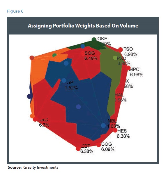
Now that the portfolio has a tangible body, we compute the volume and assign weights to every asset based on the pro rata volume contribution. The equation is simple: Volume = Money (Figure 6).
When we calculate the volume attributed to every asset, we are determining the amount of capital that is optimally allocated to those assets based on diversification and utility.
Highly correlated assets compete with each other for space in the portfolio. Intuitively, these highly correlated assets are also increasingly sensitive to small differences in their utility function. In contrast, a less correlated asset in an otherwise correlated portfolio will be relatively insensitive to changes in its utility function. If one could find a historically negatively correlated asset with positive utility, it would also be relatively insensitive to the magnitude of its utility.
The origin of the model is cash. More specifically, it is a hurdle rate that any risky investment would have to outperform to warrant consideration into the portfolio. As such, increased cash holdings are warranted in more concentrated portfolios. Cash is a drag on a well-rounded portfolio. For every potential direction in the market, a balanced portfolio contains assets with greater utility than just cash.
Diversification Weighted 500:
Performance Refinements
Here we explore some of the specific estimation techniques we have applied to the research presented. Such estimation techniques, researched over the years, represent our baseline of best practices, learned and refined from our days as a software company. We were deliberate in our attempt to balance the simplicity of the rules applied, with the robustness of the process, the applicability to diverse strategies and the final performance.

Collect the historical index component data that were in the index (S&P 500) at the start of the observation period. The data source includes delisted assets to eliminate survivorship bias.

Apply any allocation constraints and apply the investment policy to the portfolio. This fixed set of policies generates the capital market assumptions and includes data sampling, econometrics and investor preferences.

Compute the optimization (vector mapping, scaling, and volumes) to obtain the allocation weights and walk forward the test for the ensuing one-year period.

Export the computed return series and adjoin with that of other periods to create a continuous-return time series for each sector.

Repeat this process for each sector and period. Take the Diversification Weighted sector composites and optimize those using the same process to create the DW 500.
Contrast To Other
Weighting Approaches
Diversification Weighted
Equal Weighted
Fundamental Weighted
Market Cap
Revenue Weighted
Earnings Weighted
Volatility Weighted
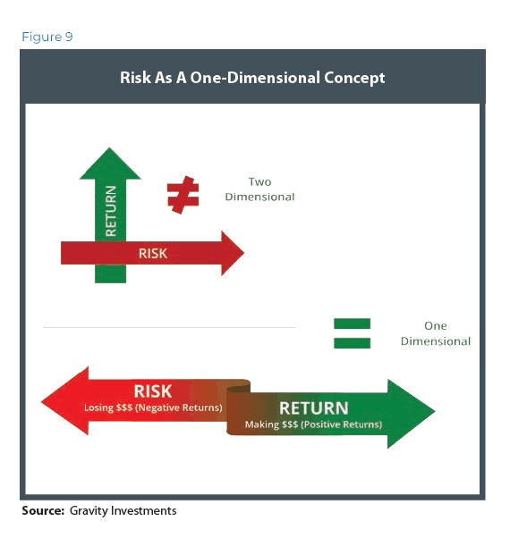
We will limit the analysis in this section to risk-based strategies, as investors may more easily confuse risk with diversification. When we talk about risk-based strategies, we include low volatility, minimum volatility, mean-variance optimization, and risk parity.
Funds of this ilk have seen recent success both in performance and garnering new assets. Now, 16 ETFs collectively manage $16 billion in funds from a strategy that did not exist before 2004. As the nature of indexation becomes more complex, the ETF market is now more accepting of smart-beta strategies. This will likely continue, but when put in context with the $2 trillion of global capital Markowitz estimated as being managed in accord with mean-variance optimization (Markowitz, private conversation, 2010), one can see the ETF space is nascent in its adoption of more complex systematic index products.
